
Manufacturing quality isn't just about catching defects after they happen. The bulk of ensuring quality lies in understanding patterns, preventing problems before they escalate, and building systems that keep quality consistent across every shift and production run.
Addressing these concerns is where Defect Density (DD) demonstrates its ability to be a reliable compass for managing quality. DD reveals trends, guides improvement efforts, and helps you connect equipment health to product quality in ways that drive real operational improvements.
In this guide, we'll walk through how to calculate, track, and use defect density to transform your quality management from reactive problem-solving to proactive quality assurance that keeps both customers and production teams confident in every product that leaves your facility.
What Is Defect Density and Why It Matters in Manufacturing
Defect Density is a quantitative metric that measures the number of defects per unit size in manufacturing, calculated by dividing the total number of defects by the size of the production unit being measured. This metric serves as a critical quality control indicator that helps manufacturing teams compare quality performance across different production runs, equipment lines, or facilities.
Unlike software development, where defect density typically refers to bugs per lines of code, manufacturing defect density focuses on physical imperfections, dimensional variations, or functional failures in produced goods. The "unit size" can vary depending on your operation. It might be per thousand units produced, per square meter of material, or per hour of production time.
Manufacturing teams rely on defect density because it provides a standardized way to track quality trends over time. When your DD starts climbing, it's often the first signal that equipment needs attention, processes are drifting, or materials are changing. This early warning system allows maintenance and quality teams to intervene before defects escalate into customer complaints or regulatory issues.
The metric becomes particularly powerful when you track it alongside equipment performance data. A sudden spike in defect density often correlates with specific machine conditions, tool wear patterns, or maintenance events, giving you clear direction on where to focus improvement efforts.
Understanding Manufacturing Defects and Their Impact
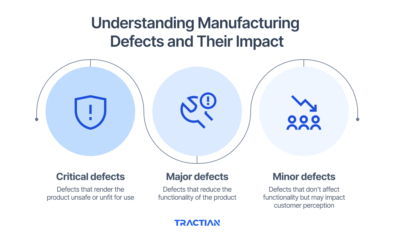
Manufacturing defects fall into three primary categories that directly influence how you calculate defect density and respond to measurements. What is defect classification all about? It starts with understanding the severity and impact of each quality failure.
Critical defects render products unsafe or completely unusable. Think of a cracked pressure vessel or a missing safety component. Major defects reduce functionality without creating safety risks, like a motor that runs but operates outside specified parameters. Minor defects don't affect performance but impact customer perception, such as surface scratches or cosmetic imperfections.
The financial impact of these defects extends far beyond the immediate cost of rework or scrap. Critical defects can trigger product recalls, regulatory investigations, and liability claims that cost millions of dollars. Major defects often result in warranty claims, customer returns, and damaged relationships with key accounts. Even minor defects accumulate costs through increased inspection time, customer complaints, and brand reputation damage.
Here's how defect categories break down in practice:
- Critical defects: Defects that render the product unsafe or unfit for use
- Major defects: Defects that reduce the functionality of the product
- Minor defects: Defects that don't affect functionality but may impact customer perception
Production delays represent another significant cost factor when defect density rises. High defect rates force teams into reactive mode, disrupting production lines, increasing inspection frequency, and diverting resources from planned maintenance to emergency fixes. This reactive cycle compounds the problem because deferred maintenance often leads to more equipment-related defects.
Defect Density Formula and Calculation Methods
The basic defect density formula provides a straightforward approach to quantifying quality performance: Defect Density = Number of Defects / Size of Production Unit. However, the real challenge lies in defining what constitutes your "production unit" and ensuring consistent measurement across your operation.
Understanding how to calculate defect density starts with getting the numerator right. The number of defects must include all quality failures detected during your measurement period, whether found during in-process inspection, final quality checks, or customer returns. Some teams make the mistake of only counting defects found at final inspection, which underestimates the true defect density and masks process problems occurring earlier in production.
The denominator varies significantly based on your manufacturing type and measurement objectives. Discrete manufacturers typically use units produced, while continuous processes might measure per ton of material processed or per hour of operation. Surface-critical operations often use area measurements like square meters, while precision manufacturing might focus on critical dimensions or features.
Different measurement approaches work better for different manufacturing environments:
Consistency in measurement timing is crucial for meaningful defect density calculations. Some defects only become apparent after aging, thermal cycling, or field use, so you need to decide whether to measure defects at production completion or after a specified time period.
Step-by-Step Defect Density Calculation Examples
Basic Calculation Example
Consider a typical stamping operation where quality inspections reveal a number of defects across the production run. The formula for defect density calculation is the number of defects divided by the total number of units produced, allowing you to express defects per unit or per a standardized quantity such as 1,000 units.
This result gives you an idea of the proportion of defective units in your production, but the real value comes from tracking this number over time. A noticeable increase in defect density often signals a process change that needs investigation. The timing coincides with a die change on Press #3, giving maintenance a clear starting point for root cause analysis.
When interpreting defect density results, consider both the absolute number and the trend direction. A defect density of 4.7 per 1,000 might be excellent for a complex assembly operation, but concerning for a simple stamping process, making industry benchmarks and historical performance your primary reference points.
Normalizing Defect Density Across Production Lines
Comparing defect density between different production lines requires normalization to account for varying complexity, cycle times, and quality requirements. A circuit board assembly line is much more complex than a simple machining operation, so comparing their defect densities directly may not provide meaningful insights.
The normalization process involves establishing a complexity factor based on the number of quality-critical operations, inspection points, or potential failure modes. For the circuit board line, you might calculate defects per 100 components rather than per unit, while the machining line uses defects per critical dimension. This approach reveals which processes truly perform better when complexity differences are factored out.
Production speed variations also require normalization when comparing lines with different cycle times. Production lines with varying speeds and precision levels encounter different quality challenges, so measuring defect density per production hour can sometimes offer a more meaningful comparison than measuring defects per unit.
What Is a Reasonable Defect Density Target?
Many manufacturers strive for very low defect densities in critical components and processes, but what counts as a reasonable defect density can vary significantly depending on product complexity, industry standards, and the importance of the application. Defect density requirements can vary significantly depending on the industry and application, with more critical components typically requiring stricter quality standards than consumer goods.
Industry benchmarks provide starting points, but your specific targets should reflect customer requirements, regulatory standards, and cost of quality considerations. A medical device manufacturer faces different quality expectations than a furniture producer, making industry-specific benchmarks more relevant than generic manufacturing targets.
Setting appropriate defect density targets requires balancing quality costs with quality benefits. Reducing defect density from higher to lower levels often requires additional investment in inspection and process controls. Regardless, these efforts can lead to substantial savings by minimizing warranty claims and customer returns. However, reducing defect density from 100 to 10 parts per million often requires significant investment, which may not always be justified by the potential reduction in associated losses.
Product complexity directly influences achievable defect density levels. Generally, simpler parts with fewer critical dimensions are less prone to defects compared to complex assemblies with many components and potential failure modes. Your targets should reflect this complexity while still driving continuous improvement.
Defect Rate Versus Defect Percentage and Other Quality Metrics
Defect density, defect rate, and defect percentage measure different aspects of quality performance and serve complementary roles in a comprehensive quality monitoring system. Understanding these defect metrics helps you choose the right measurement for each situation.
The defect rate typically expresses defects per unit time (defects per hour or per day), while defect percentage shows the proportion of defective units in a production lot. These metrics provide different insights into quality performance patterns. Defect density helps normalize quality across varying production volumes, defect rate reveals how quality changes with production speed or shift patterns, and defect percentage shows the immediate impact on customer shipments.
First pass yield measures the percentage of units that pass all quality checks without rework, providing insight into process capability and efficiency. While defect density focuses on the number of problems found, first pass yield emphasizes successful production, making it valuable for tracking improvement initiatives and operational efficiency.
Key quality metrics work together to provide comprehensive visibility:
A defect rate calculator can help automate these calculations, but understanding the underlying formulas ensures you're measuring what matters most for your operation.
Escaped Defects and Defect Escape Rate in Manufacturing
Escaped defects represent quality failures that pass through all internal inspection points undetected. When these reach customers, they create the most costly and damaging quality problems. The defect escape rate measures the percentage of total defects that escape your quality control system, providing critical insight into inspection effectiveness.
Understanding both internal defect density and escaped defects gives you complete visibility into quality performance. You might have high defect density measurements, but with excellent internal defect detection, customer satisfaction remains high. Conversely, even if internal defect density is low, high escape rates indicate inspection gaps that need immediate attention. Otherwise, customer satisfaction will be at risk.
Customer returns, warranty claims, and field failure reports provide the data needed to calculate defect escape rates. However, this data often arrives weeks or months after production, making real-time escape rate monitoring challenging. Some manufacturers use accelerated testing or extended internal inspection periods to estimate escape rates more quickly.
Calculating Defect Escape Rate
The defect escape rate formula divides escaped defects by total defects (internal plus escaped): Escape Rate = Escaped Defects ÷ (Internal Defects + Escaped Defects).
For example, if you track both internal defects and those reported by customers from the same production period, you can calculate your escape rate by dividing the number of escaped defects by the total number of defects found both internally and externally.
This calculation requires careful timing alignment between internal defect detection and customer feedback. Defects found during production should be matched with customer reports from the same time period, accounting for shipping delays and customer usage patterns that affect when problems are discovered and reported.
Tracking escape rates by defect type reveals weaknesses in the inspection system. If dimensional defects rarely escape but functional defects frequently reach customers, your measurement systems might be adequate, while your performance testing needs improvement.
Reducing Escaping Defects Through Process Improvements
Reducing escaping defects requires both better defect prevention and improved defect detection. Process improvements that reduce overall defect density automatically reduce escaped defects, while inspection improvements catch more defects before they reach customers.
Statistical process control techniques help prevent defects by maintaining process parameters within control limits. When combined with real-time monitoring systems, these approaches catch process drift before it generates defects, reducing both internal defect density and escape rates simultaneously.
Inspection system improvements focus on detection capability and coverage. Adding inspection points, upgrading measurement equipment, or implementing automated inspection systems can significantly reduce escape rates. However, the investment must be justified by the cost of defects that escape to customers.
Implementing a Defect Density Monitoring System
Successful defect density monitoring requires systematic data collection, consistent analysis methods, and clear action protocols that turn measurements into improvements. The system must capture defects at multiple inspection points while maintaining data integrity and providing timely feedback to production teams.
Data collection methods range from manual inspection logs to automated vision systems, but consistency matters more than sophistication. The key is establishing clear defect definitions and training inspectors to apply them consistently.
Measurement frequency depends on production volume and process stability. High-volume operations might require hourly defect density calculations to catch problems quickly, while low-volume precision manufacturing might use daily or weekly measurements. The frequency should provide early warning of quality problems without overwhelming teams with data.
Data Collection Best Practices
Effective defect data collection starts with clear, unambiguous defect definitions that eliminate inspector subjectivity. Each defect category needs specific criteria, measurement methods, and examples that ensure consistent classification across shifts and inspectors. Visual standards with photographs or physical samples help maintain consistency.
Automated data collection systems reduce human error and provide real-time defect density calculations, but they require careful setup and validation. Vision systems must be trained on actual production defects, not laboratory samples, and their performance should be verified regularly against human inspection to ensure accuracy.
Inspection point placement affects the types of defects you detect and when you detect them. Early inspection points catch process problems quickly, but might miss defects that develop during subsequent operations. Final inspection catches all defects but provides delayed feedback that limits the effectiveness of corrective action.
Using Defect Density to Drive Continuous Improvement
Defect density data becomes most valuable when it drives specific improvement actions rather than just monitoring performance. Root cause analysis of defect density spikes should lead to corrective actions that prevent recurrence, while trend analysis guides long-term improvement initiatives.
Pareto analysis of defect types helps prioritize improvement efforts by focusing on the defects that contribute most to overall defect density. Solving the top three defect causes might reduce total defect density by 70%, providing a better return on improvement investment than addressing all defect types equally.
Cross-functional improvement teams use defect density data to guide process changes, equipment upgrades, and training initiatives. When maintenance, quality, and production teams share defect density data and responsibility for improvement, solutions address root causes rather than symptoms.
Improving Defect Density Through Better Maintenance Practices
Equipment condition directly impacts defect density through tool wear, calibration drift, and mechanical degradation that gradually increases quality problems.
Predictive maintenance strategies that monitor equipment health can prevent many defect-causing failures before they affect production quality.
Preventive maintenance scheduling based on defect density trends provides early warning of equipment problems. When defect density starts increasing on a specific production line, scheduled maintenance can address developing issues before they cause significant quality problems or equipment failures.
Condition-based maintenance uses real-time equipment monitoring to optimize maintenance timing and prevent defect-causing failures. Vibration analysis, thermal monitoring, and oil analysis can detect equipment degradation that leads to quality problems, allowing maintenance intervention before defects increase.
Root cause analysis of defect-causing equipment failures helps prevent recurrence and guides improvements to maintenance strategies. When a bearing failure causes dimensional defects, analyzing the failure mode helps prevent similar problems on identical equipment throughout the facility.
How Tractian CMMS Elevates Defect Density Management
Manufacturing teams serious about reducing defect density need more than just measurement systems. They need integrated maintenance strategies that prevent the problems causing quality issues. Tractian CMMS provides the foundation for connecting equipment health to quality performance through systematic maintenance planning and execution.
When defect density starts climbing, Tractian CMMS helps teams quickly identify which equipment might be contributing to quality problems through comprehensive asset history tracking and failure analysis tools. Work orders automatically capture the relationship between maintenance activities and subsequent quality performance, building a database that reveals which maintenance actions most effectively reduce defects.
The platform's preventive maintenance scheduling ensures that defect-critical equipment receives attention before problems develop. Instead of waiting for defect density to spike, teams can maintain equipment based on proven schedules that keep quality performance stable and predictable. This proactive approach transforms defect density from a reactive measurement into a strategic management tool.
With automated reporting and trend analysis, quality and maintenance teams can spot developing problems early and take corrective action before defects impact customers or production efficiency. The system helps teams move beyond firefighting to build systematic approaches that prevent quality problems at their source.
Ready to connect your maintenance strategy with quality performance?
Start a free trial and see for yourself how Tractian CMMS helps manufacturing teams reduce defect-causing equipment failures and maintain consistent quality standards.